A functional connectome containing 200,000 cells, 75,000 neurons with physiology, and 523 million synapses.
This resource provides interactive visualizations of anatomical and functional data that span all 6 layers of mouse primary visual cortex and 3 higher visual areas (LM, AL, RL) within a cubic millimeter volume.

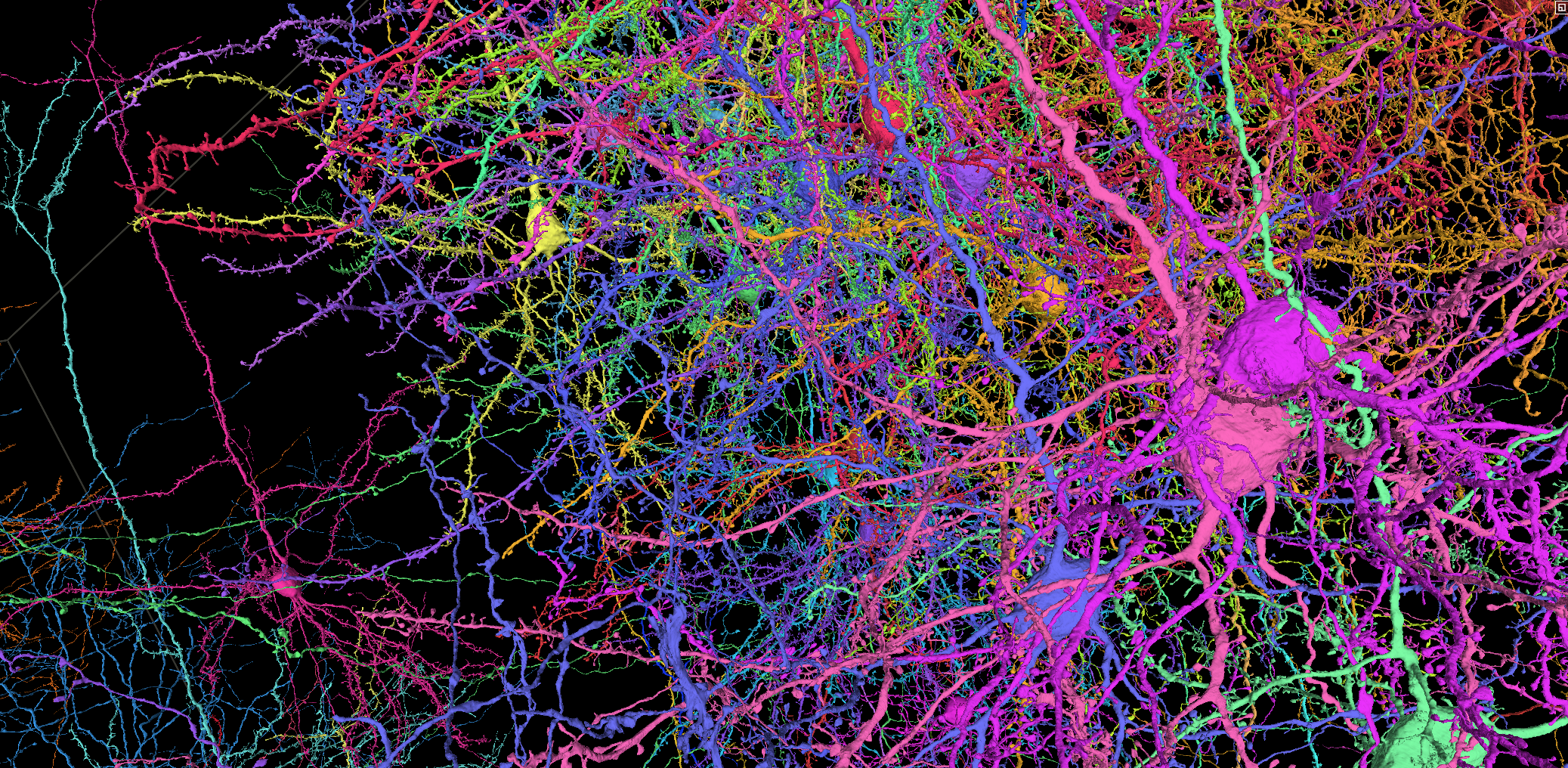
Screenshot of neuroglancer data visualization in browser. Click the image to jump to this live view of pyramidal neurons
When accessing the dynamic segmentation for the first time, you may need to accept the Terms of Service (authorize with any google account)
A functional connectomics dataset spanning multiple visual areas.

This IARPA MICrONS dataset spans a 1.4mm x .87mm x .84 mm volume of cortex in a P87 mouse. It is 400x larger than the previously released Phase 1 dataset, which can be found here. The dataset was imaged using two-photon microscopy, microCT, and serial electron microscopy, and then reconstructed using a combination of AI and human proofreading.
Functional imaging data of an estimated 75,000 pyramidal neurons in the volume contains the single cell responses to a variety of visual stimuli. That same tissue was imaged with high resolution electron microscopy and processed through a machine learning driven reconstruction pipeline to generate a large scale anatomical connectome. The anatomical data contains more than an estimated 200,000 cells, and 120,000 neurons (details). Automated synapse detection measured more than 523 million synapses.
This makes this dataset remarkable in a few key ways:
It is the largest multi-modal connectomics dataset released to date and the largest connectomics dataset by minimum dimension, number of cells, and number of connections detected (as of 2025)
It is the first EM reconstruction of a mammalian circuit across multiple functional brain areas.
Below you can find visualization tools, as well as instructions and links to tutorials for how to query and download portions of the dataset programmatically. To “git started” analyzing data, checkout the MICrONS Programmatic Tutorials for anatomical data and the MICrONS Neural Data Access (NDA) repository for functional data.
The paper with details about the dataset is published at Nature:
The MICrONS Consortium, et al. 2025. “Functional Connectomics Spanning Multiple Areas of Mouse Visual Cortex.” Nature 640 (8058): 435–47. https://doi.org/10.1038/s41586-025-08790-w.
See more under Publications.
Use Cases

Cell Types
You can use this dataset to explore the morphology and connectivity of a very diverse variety of excitatory, inhibitory, and non-neuronal cell types throughout the volume.
Click these links for example cells:bipolar cells, basket cells, a chandelier cell, martinotti cells, a layer 5 thick tufted, a layer 5 NP cell, layer 4 cells, layer 2/3 cells, blood vessels, astrocytes, microglia. For programmatic access of more systematic cell type information released thus far, explore MICrONS Tutorials.

Synaptic Connectivity
Query from hundreds of millions of synapses in the volume from any of the segmented cells. To see an example visualization with one cell’s inputs and outputs annotated click the button below. We are releasing an app that you can use to query this data non-programmatically and generate a synaptic visualization for any cell. To learn how to query the data programmatically yourself, look at this notebook on MICrONS Tutorials.

Functional Data
All the functional recordings from 115,372 regions of interest and 75,902 estimated neurons are available, including the response of those units to a variety of visual stimuli. You can download the database of functional recordings to explore how cells responded to visual stimuli. For a subset of the neurons, we have generated a correspondence between their functional recording and their anatomical reconstruction. To learn how to query the functional databases and link them to the anatomical data, you can view this notebook on MICrONS NDA, or access a hosted database and interactive notebooks by following the instructions at this repository.
Besides the interactive visualization of the imagery and flattened static segmentation above, we are making access available to tools that facilitate querying and updating of the data programmatically via python. Details on how to access different aspects of the data are listed below by category.

Electron Microscopy Imagery
Synaptic Connectivity

Nucleus Segmentation

Functional Co-Registration

Vasculature Segmentation

Cell Segmentation
Proofreading Status

Neuron Skeletons
Digital Twin Functional Model

Cell Meshes

Cell Types

Functional Data

Functional Connectomics Analysis
Anatomical Data
Multiple cloud providers have graciously agreed to host and share MICrONS data in public buckets. This includes Amazon Web Services thanks to the Amazon Public Datasets program, as well as from within Google Cloud, thanks to the Connectomics at Google team.
Cloud-volume can be used to programmatically download EM imagery from either location with the cloud paths below.
The JHU-APL team is also providing the images available via their BossDB service which you can be accessed via the python client intern. Find more details about how to access this dataset via BossDB here.
The imagery was reconstructed in two portions, referred to internally by their nicknames ‘minnie65’ and ‘minnie35’ reflecting their relative portions of the total data. The two portions have now been aligned across an interruption in sectioning.
minnie65:
AWS Bucket: precomputed://https://bossdb-open-data.s3.amazonaws.com/iarpa_microns/minnie/minnie65/em
Google Bucket: precomputed://https://storage.googleapis.com/iarpa_microns/minnie/minnie65/em
minnie35:
AWS Bucket: precomputed://https://bossdb-open-data.s3.amazonaws.com/iarpa_microns/minnie/minnie35/em
Google Bucket: precomputed://https://storage.googleapis.com/iarpa_microns/minnie/minnie35/em
As with images, cloud-volume and intern can be used to download voxels of the cellular segmentation from the below locations. Although the images are now aligned, minnie65 was segmented first and has undergone significant proofreading.
There are presently 8 publicly available versions of the release: versions 117, 343, 661, 785, 943, 1078, 1181, and 1300 (see more about public data releases in the Manifests page).
Static segmentation: The version 117 (June 11, 2021), 343 (February 22, 2022), and 943 (January 22, 2024), and 1300 (January 13, 2025) minnie65 segmentations are available as ‘flattened’ snapshots of the state of proofreading that include multiple resolutions for rendering and download.
Dynamic segmentation: Ongoing releases of the segmentation are available available as a dynamic agglomeration of the watershed layer, under the datastack name “minnie65_public” of which version 1300 (January 13, 2025) is the latest. This format includes access to the entire edit history of the segmentation.
minnie65_public dynamic segmentation: (presently version 1300)
PyChunkedGraph location: graphene://https://minnie.microns-daf.com/segmentation/table/minnie65_public
Version 117 static segmentation
Google bucket: precomputed://https://storage.googleapis.com/iarpa_microns/minnie/minnie65/seg
AWS bucket: precomputed://https://bossdb-open-data.s3.amazonaws.com/iarpa_microns/minnie/minnie65/seg
Version 343 static segmentation
Google bucket: precomputed://https://storage.googleapis.com/iarpa_microns/minnie/minnie65/seg_m343/
Version 943 static segmentation
Google bucket: precomputed://https://storage.googleapis.com/iarpa_microns/minnie/minnie65/seg_m943/
Version 1300 static segmentation
Google bucket: precomputed://https://storage.googleapis.com/iarpa_microns/minnie/minnie65/seg_m1300/
The minnie35 segmentation has not undergone any proofreading and is being released as is.
minnie35:
Google bucket: precomputed://https://storage.googleapis.com/iarpa_microns/minnie/minnie35/seg
AWS bucket: precomputed://https://bossdb-open-data.s3.amazonaws.com/iarpa_microns/minnie/minnie35/seg
In addition you can download the ground truth segmentation data that was generated for this dataset as part of this archive (1.1Gb) as part of this zenodo dataset.
The static cell segmentation voxels were meshed by the Connectomics at Google team into a multi-resolution sharded mesh format. The cloud paths for the voxel segmentation can be used to access these meshes with cloud-volume.
Although the static segmentation reflects the state of proofreading at the time of the release, there are aspects of the static meshes which can be unintuitive. In particular, gaps in the segmentation and mesh can occur at locations where false splits were corrected. Also, locations where a neuron contacts itself, such as an axon coming in contact with a dendrite of the same cell, can be merged in the mesh. This can make some types of morphological analysis of these meshes challenging. To address this, we are also making available dynamic meshes that were calculated and backed by our proofreading infrastructure CAVE (Connectome Annotation Versioning Engine). These meshes have only one resolution, but more accurately reflect the topology of the neuron by not over-merging meshes. You can further process and repair the meshes to fill gaps and make ‘watertight’ with MeshParty the mesh processing library we have developed.
To access these meshes you must register as a CAVE user for the microns public dataset. A tutorial on using accessing both types of meshes can be found on the MICrONS Tutorials pages.
Dynamic mesh paths:
minnie65: graphene://https://minnie.microns-daf.com/segmentation/table/minnie65_public
minnie35: graphene://https://minnie.microns-daf.com/segmentation/table/minnie35_public_v0
To query synaptic connectivity, you need to register as a user in the CAVE (Connectome Annotation Versioning Engine) infrastructure. To do so, visit this page.
Once registered, you can use the CAVEclient, to query many aspects of the data as annotation tables, including synapses. A tutorial on how to do this can be found here. At present we only have queryable synapses from the larger proofread volume available.
Alternatively, one can non-programatically query and visualize inputs and outputs of synapses from individual cells using the the Connectivity Viewer.
A cell can be queried by its nucleus ID (see below), or its segmentation ID in this version. The nucleus ID identifies the cell based upon its soma location and will more accurately track cells with cell bodies across versions of the dataset. An individual segmentation ID could contain 0, 1, or more than 1 cell bodies and there will be a new ID assigned when objects are merged or split.
For large scale downloads of all synapses, see bulk data access.

We have developed an automated segmentation method of the nuclei within the volume. The voxelized segmentation and flat meshes can be accessed using the below buckets using cloud-volume or intern, and can be added as a layer in neuroglancer. Example link.
minnie65:
AWS Bucket: precomputed://https://bossdb-open-data.s3.amazonaws.com/iarpa_microns/minnie/minnie65/nuclei
Google bucket: precomputed://https://storage.googleapis.com/iarpa_microns/minnie/minnie65/nuclei
A nucleus segmentation of the smaller section of the dataset is not yet available.
The CAVEclient can be used to query an annotation table called ‘nucleus_detection_v0’, which contains the location and volume of each of these detections, including what segmentation ID underlies those detections. See this the MICrONS Tutorials for an example.
Beginning in v661, an additional check was run to check if the centroid location of the nucleus was in fact inside the nucleus and inside the segmentation. If either was not true, an algorithm searched in a 15 micron cutout for a location that was inside the nucleus segmentation and inside the cellular segmentation, as an alternative location to associate the nucleus with a cellular segmentation object. This resulted in 8,388 nuclei with alternative lookup points, which are available in the table called ‘nucleus_alternative_points’.
A merge of the original table with the alternative points overriding it is available as a ‘view’ called ‘nucleus_detection_lookup_v1’ from the CAVEclient starting v661.
Note: An effort was made to use the nucleus segmentation to ensure that the nucleus of each cell is merged with the cytoplasm of the cell, but this was not in all cases successful, particularly for cells with fragmented segmentations. In such cases, querying the segment that underlies the centroid of nucleus detection can return a segment which is an unmerged nucleus of a cell.
The automated segmentation is good, but not perfect, and can be improved with human intervention. A concerted effort was made to do proofreading on a subset of neurons within the dataset, in addition, proofreading can be focused on dendrites or axons, and to varying levels of completeness.
We are releasing a list of of cells which have undergone varying levels of proofreading as an annotation table proofreading_status_and_strategy. See details at Proofreading and Data Quality
For an example of how to access the proofreading data, see this example in the MICrONS Tutorials
Identifying the putative ‘cell type’ from the EM morphology is a process that involves both manual and automatic classifications. Subsets of the dataset have been manually classified by anatomists at the Allen Institute, and these ground truth labels used to train and refine different automated ‘feature classifiers’ over time.
The diversity of manual and automated cell type classifications available in the dataset reflect the fact that definitions of ‘cell types’ in the dataset is an active area of research and must be contextualized against the purpose and resolution of the cell-typing being performed.
Manual Cell Types (V1 Column)
A subset of nucleus detections in a 100 um column (n=2204) in VISp were manually classified by anatomists at the Allen Institute into categories of cell subclasses, first distinguishing cells into classes of non-neuronal, excitatory and inhibitory. Excitatory cells were separated into laminar sub-classes (L23, L4), 3 sub-types of layer 5 cells (ET, IT, NP) and 2 classes of layer 6 cells (IT, CT). Inhibitory cells were classified into Bipolar (BPC), Basket (BC), Martinotti (MC), or Unsure (Unsure). Those neuronal calls are available from the CAVEclient under the table name allen_v1_column_types_slanted_ref which references the nucleus id of the cell.
Non-neuronal manual cells type calls enumerate astrocytes, microglia, pericytes, oligodendrocytes (oligo), and oligodendrocyte precursor cells (OPC), and area available in the table aibs_column_nonneuronal_ref.
Unsupervised Clustering (m-types)
Unsupervised clustering analysis as described in Schneider-Mizell et al., Nature 2025, created automated labels on these Column Neurons. The inhibitory subclass clusters are annotated based on their broad connectivity statistics: ITC (interneuron targeting cell), PTC (proximal targeting cell), DTC (distal targeting cell), and SPC (sparsely targeting cell). Excitatory cells clusters are annotated based on their layer and subtype. See the paper for more details.
V1 Column Predictions
M-type predictions for the Column Neurons are available in the table allen_column_mtypes_v2. As described in the paper, further clustering of the inhibitory cells based on their cell type specific connectivity patterns grouped them into 20 orthogonal connectivity motifs which are available in the table connectivity_groups_v795.
Dataset-wide predictions
This model was further refined with the soma-nucleus Cell Type labels described below, and the ‘metamodel’ of the two classifications was run for all neuron-nucleus detections in the dataset. This is available as table aibs_metamodel_mtypes_v661_v2
Cell Type classification (Soma-nucleus models)
Models were trained based upon the manual Column Neuron labels, as described in Elabbady et al. Nature 2025. Each nucleus was analyzed for a variety of features, and a model trained on and independent dataset to distinguish neurons from non-neuronal detections. Non-neuron detections include both glial cells and false positive detections. The nucleus segmentation detected 171,818 connected components of nucleus objects, this model detected 82K neurons. Evaluation of this model on 1,316 cells in the volume shows the model has a recall of 99.6% for neurons, and a precision of 96.9%. All nucleus detections and the results of this model can be queried and linked to the cellular segmentation using the CAVEclient with the table name nucleus_neuron_svm.
An example analysis can be found in the MICrONS Binder. Nucleus detections of less than 25um^3 were generally false positives, but the volume of each detection larger than that is also available in the table nucleus_detection_v0. Glial and epithelial cells are highly enriched within non-neurons of >25um^3 but some false detections remain.
For the neurons, we further extracted features of the ultrastructure surrounding the somatic region of the cell, including its volume, surface area, and density of synapses. Combining those features with the nucleus features we trained a hierachical model on the labels from allen_v1_column_types_slanted_ref and aibs_column_nonneuronal_ref to predict cell-classes and sub-classes across a large number of neurons.
V1 Column Predictions
These prediction are described in the paper and are available in the table named aibs_soma_nuc_metamodel_preds_v117. A similar model was trained using the labels from allen_column_mtypes_v1 and those results are available in the table named aibs_soma_nuc_exc_mtype_preds_v117. (Available in v343 and v661 of the public dataset)
Dataset-wide predictions
The refined model, incorporating the m-type labels described above, as the ‘metamodel’ of the two classifications was run for all nucleus detections (including non-neuronal) in the dataset. This is available as table aibs_metamodel_celltypes_v661.
Excitatory/inhibitory classification
An alternative approach was applied to a subset of cells as described in Celii B. et al. Nature 2025. Briefly, spine density was calculated on individual neurons and used to train a logistic classifier as to whether they were likely inhibitory and excitatory. These results are available in a table named baylor_log_reg_cell_type_coarse_v1. In addition, finer cell type labels based were predicted using a graph neural network on a skeleton-like representation of the neuron that included features extracted from the segmentation. The result of this classifier are available in a table called baylor_gnn_cell_type_fine_model_v2. (Available in and v661 and v943 of the public dataset)
For examples querying different cell types programmatically, see the MICrONS Tutorials.

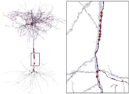
Three renderings of the same neuron: skeleton, skeleton with compartment labels and radius scaling, meshwork skeleton with synapse annotations
We have pre-generated skeletons and Meshworks available for neurons from version 661 of the MICrONS dataset.
Most of the included h5, json and swc files represent excitatory neurons’ dendrite and soma morphologies that have been automatically reconstructed with little to no human proofreading. These span much of the millimeter cubed of the MICrONS dataset except for the edges where the majority of the morphology would be cut off. There is a smaller subset of manually-proofread excitatory and inhibitory neurons with axons, dendrite and soma reconstruction. This information is accessible in the json files.
BossDB repository: s3://bossdb-open-data/iarpa_microns/minnie/minnie65/skeletons/v661/
Skeleton
Access from: s3://bossdb-open-data/iarpa_microns/minnie/minnie65/skeletons/v661/skeletons
The swc files contain a simple graphical representation of neurons that has nodes with their 3d points in space, the estimated radius of those points and the compartment of the node (axon, (basal) dendrite, apical dendrite, soma).
Meshwork
Access from: s3://bossdb-open-data/iarpa_microns/minnie/minnie65/skeletons/v661/meshworks
h5 file here can be ingested into a meshwork object in python with the package MeshParty. This meshwork integrates anatomical data and other user defined annotations such as synapses. The meshworks here contain annotation tables including pre and post synaptic chemical synapses on the given neuron and the ids of the post or presynaptic neurons respectively. Unless the neuron has had a high level of proofreading, the axon has been masked and removed.
Metadata Json
Access from: s3://bossdb-open-data/iarpa_microns/minnie/minnie65/skeletons/v661/metadata
json files contain metadata and various features of the neuron skeleton including the proofreading version of the microns dataset, the various ids of the given body, and information on masked out indices.
The variables included in the Json file are:
| Variable name | Description |
|---|---|
soma_location |
location of the center of the soma for the given neuron in voxels |
soma_id |
identification number of the soma nucleus of the given neuron |
root_id |
identification number (segmentation id) of this specific version of this neuron. If the given neuron undergoes proofreading and some neuron segment is added or removed, it will be given a new root it. The root id recorded here was the root for this neuron in the current version (see ‘version’ value in this meta file) |
supervoxel_id |
identification number of a supervoxel (smallest unit of segmentation) at the center of the soma of the given neuron |
version |
MICrONS dataset materialization version from which the meshwork and skeleton was generated from. Different versions have different level of proofreading |
apical_noes |
indices of excitatory skeleton nodes in this neuron that have been predicted to be apical nodes. Per the system we used, there could be no apicals, one apical, or multiple apicals. One apical is the most common |
basal_nodes |
indices of excitatory skeleton nodes predicted to be basal dendrites |
true_axon_nodes |
Only measured in the highly proofread neurons for which we retained the axons on the skeletons. Indicates the indices of skeleton nodes that represent the axon. Compare to classified_axon_nodes below, and additional metadata on the proofreading status |
total_skeleton_path_length |
total cable length of skeleton (in nm) |
apical_length |
total cable length of apical nodes along skeleton (in nm) |
basal_length |
total cable length of basal nodes along skeleton (in nm) |
axon_length |
total cable length of axon nodes along skeleton (in nm) |
percent_apical_pathlength |
(apical_length/total_skeleton_path_length)*100 |
percent_basal_pathlength |
(basal_length/total_skeleton_path_length)*100 |
percent_axon_pathlength |
(axon_length/total_skeleton_path_length)*100 |
classified_axon_nodes |
indices of skeleton nodes that were predicted to be axons by algorithm, but were not removed during peel-back due to having a downstream segment that was identified as a dendrite. (A measure of potential error in the compartment labeling process) |
length_remaining_classified_axon |
total cable length of skeleton nodes that were predicted to be axons by algorithm, but were not removed due to having a downstream segment that was identified as a dendrite. (A measure of potential error in the compartment labeling process) |
percent_remaining_classified_axon_pathlength |
(total_classified_axon_pathlength/total_skeleton_path_length)*100 |
The Json metadata files also include the proofreading status indicators for the cells, which determined whether the axon was excluded from skeletonization and compartment labeling. These metrics are as follows:
| Variable name | Description |
|---|---|
tracing_status_dendrite |
indicates the amount and mode of proofreading that has been conducted on the dendrite of the neuron. May be one of: non, clean, extended. See Proofreading Strategies for more information. |
tracing_status_axon |
indicates the amount and mode of proofreading that has been conducted on axon of the neuron. May be one of: non, clean, extended. See Proofreading Strategies for more information. |
tracing_pipeline |
indicates if axon is included or has been masked out/removed from the meshwork and skeletons |
clean_axon_included |
indicates that the neuron has been sufficiently proofread and that the axon has not been removed and has been included in the skeleton and not masked over in the meshwork. There are 373 such neurons in this collection. |
all_axon_removed |
indicates that the neuron has not been sufficiently proofread, meaning the axon is not biologically accurate and has therefor been masked and removed. Asterisk indicates that this process may not have removed or masked out all the axon. See classified_axon_nodes above. |
We have developed a skeleton plotting and utility Python package called skeleton_plot. This is the library that was used to create the skeleton visualization on this page.
For examples downloading skeletons at Version 1300, see the MICrONS Tutorials: Download Skeletons
Functional Data and Co-Registration

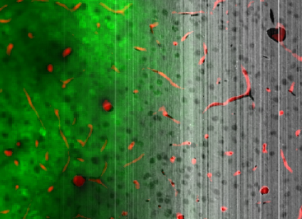
An example scan field with segmentation masks and a synchronized stimulus can be viewed interactively here. Scroll over the stimulus on the right to move forward through time.
The scan and stack metadata, synchronized stimulus movies, synchronized behavioral traces, cell segmentation masks, calcium traces, and inferred spikes are available as a containerized MYSQL v5.7 database, schematized using DataJoint. This file is available for download here (97 GB).
Instructions for using the container are available at https://github.com/cajal/microns-nda-access.
The DataJoint schema and tutorials for interacting with the data are available at https://github.com/cajal/microns_phase3_nda.
To begin exploring these data, you can get access to a hosted database and interactive notebooks by following the instructions at this repository.
Technical documentation for the database is available for download here.
The raster- and motion-corrected functional scan tiffs are available for download at:
AWS Bucket: s3://bossdb-open-data/iarpa_microns/minnie/functional_data/two_photon_functional_scans
google bucket: gs://iarpa_microns/minnie/functional_data/two_photon_functional_scans
Technical documentation
Lastly, the stitched and temporally aligned stimuli for each scan are available for download at:
AWS Bucket: s3://bossdb-open-data/iarpa_microns/minnie/functional_data/stimulus_movies
google bucket: gs://iarpa_microns/minnie/functional_data/stimulus_movies
Technical documentation
Each scan plan was registered into the two-photon structural stack via a 3d affine transformation. A visualization of all the scan fields represented as static images and registered into the structural stack can be viewed here. Note that because the planes are not all orthogonal, and they are quite dense the pattern of borders can be confusing.
Correspondence points between the two-photon structural in vivo imaging volume and EM volume were manually placed, and a 3D cubic spline transform was performed to align the two volumes. The correspondence points, transform algorithm, and solution to this transform are available at https://github.com/AllenInstitute/em_coregistration/tree/phase3. A copy of the transform solution is also stored inside the DataJoint schema above.
A custom interface was built for exploring the co-registered volumes and to facilitate manual matching between neurons from electron microscopy (EM) and units from two-photon (2P) functional scans. As of version 1300, the CAVE database contains 19,181 manual matches available in table coregistration_manual_v4. Since individual EM neurons may appear in multiple functional scans, there are 15,439 unique neurons represented in this match table. In addition to manual matching, two automated approaches were developed, producing two additional match tables described in the publication. The first automated approach used manually placed fiducials to determine transformations between EM and 2P volumes, with resulting matches available in coregistration_auto_phase3_fwd_v2. The second automated approach used the blood vessels between the two volumes for the transformation, with the resulting matches found in table apl_functional_coreg_vess_fwd. In the publication, these tables were unified by performing a merge on the common attributes: session, scan_idx, field, unit_id, target_id, in effect keeping only the “agreement” matches common to both tables. Information on methods for filtering these tables based on the confidence metrics can be found in the publication. An alternative unification approach that is not described in the publication resolves disagreements by selecting the match from the automated table with the higher confidence, based on the residual metric. This table can be found at coregistration_auto_phase3_fwd_apl_vess_combined_v2. More on this approach can be found in the table description on CAVE. To see how to query the functional data from a functionally matched cell, read this notebook in the MICrONS NDA repo.
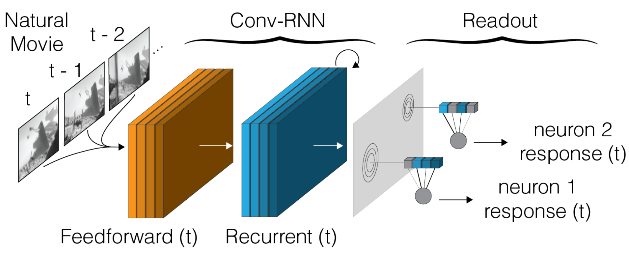
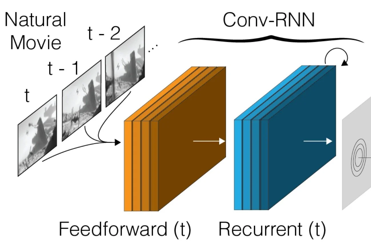
A deep neural network model trained to predict visual responses has been applied to the functional recordings in the MICrONS dataset. This model predicts neural activity in response to the visual stimuli, and also estimates important visual properties of these neurons. This includes fits of their orientation and direction selectivity, as well as an estimate of their receptive field locations.
For full details on the models and methodology and interpretations, reference:
Foundation Model of Neural Activity Predicts Response to New Stimulus Types (Wang et al., Nature 2025)
Functional connectomics reveals general wiring rule in mouse visual cortex (Ding et al., Nature 2025)
For instructions on how to download and run the model, as well as train readout feature weights for new data, please see https://github.com/cajal/fnn.
Computed properties derived from the model are available at this directory:
s3://bossdb-open-data/iarpa_microns/minnie/functional_data/digital_twin_properties/v2/ (total 32 GB)
These computed properties include:
Readout feature weights and readout locations
Performance metrics
Orientation and direction selectivity metrics
Predicted neural responses and the stimuli that generated them
Anatomical information for predicted neurons
For tutorials on downloading and using computed properties, please see https://github.com/cajal/fnn.
A subset of the above properties are available for matched functional units in the following CAVE tables:
digital_twin_properties_bcm_coreg_v4(manual matches from CAVE tablecoregistration_manual_v4)digital_twin_properties_bcm_coreg_auto_phase3_fwd_v2(automatic matches from CAVE tablecoregistration_auto_phase3_fwd_v2)digital_twin_properties_bcm_coreg_apl_vess_fwd(automatic matches from CAVE tableapl_functional_coreg_vess_fwd)
Computed properties from an earlier version of the model (now deprecated) are available at this directory:
s3://bossdb-open-data/iarpa_microns/minnie/functional_data/digital_twin_properties/v1/ (total 32 GB, readme)

The data from the functional connectomics analysis described in Ding et al. 2025, is released on bossdb:
s3://bossdb-open-data/iarpa_microns/minnie/functional_data/functional_connectomics/node_and_edge_properties/v1/
For instructions and code please see: https://github.com/cajal/microns-funconn-2025
MICrONS Explorer is pleased to advertise a separate vasculature segmentation from Jia Wan and Donglai Wei, “TriSAM: Tri-Plane SAM for zero-shot cortical blood vessel segmentation in VEM images.” (https://arxiv.org/html/2401.13961v2).
The segmentation is assessed across the entire volume (65 and 35 portions) at a resolution of 320× 256×256 nm. The segmentation is visualizable in neuroglancer, and the precomputed segmentation and mesh are downloadable from BossDB https://bossdb.org/project/wan2024
Precomputed segmentation: s3://bossdb-open-data/wei2024/minnie/bv
For large scale bulk downloads of the data, including imagery, segmentation, or meshes should use the google or AWS bucket locations. The buckets also contain static snapshots of synapse locations, nucleus detection locations, coregistration points, along with the functional data described below.
A complete manifest of the files that can be downloaded can be found under Static Repositories.
Looking Ahead
This dataset is both large in size and rich in the different types of analysis one can do. There are some directions the consortium is already working on, including:
Proofreading: There are ongoing proofreading efforts including both manual and automated efforts (see below). We will be releasing new versions of the dataset on a regular interval through the dynamic CAVE services. The static flat segmentation and files will be updated less regularly. If you would be interested in receiving notifications about updates to the dataset or are interested in proofreading the dataset, please reach out with a Vortex Request (an NIH funded mechanism by which we provide continued support for this dataset)
Cell typing: We are actively working on describing the cell types we see in the dataset through a variety of methods. As we gain confidence in the results of these analyses we will release more data annotations with finer grained cell type calls and/or predictions.
Co-registration: The final step of coregistration is presently a manual process and is ongoing. As we increase the number of high-confidence matches, they will be released.
There are other areas where there is a clear opportunity for the community to contribute. For example:
Synapse types: We do not presently have automated calls on synapse types, such as which are excitatory and which are inhibitory.
Automated proofreading: The consortium has a number of projects ongoing in trying to improve the segmentation results through automated means. For example, we have developed an automated method to identify and remove various kinds of merge errors, and expect to apply this method throughout the volume in the near future. However there are a diverse set of potential approaches and we cannot pursue all of them. Through CAVE it is possible to query the history of edits that were made to the segmentation, which can be used to train and evaluate automated approaches.
Detecting other ultrastructural features: There are many un-annotated aspects of the data. We, for example, developed models for detecting mitochondria (see: mitochondria ground truth in L2/3 dataset), but have not had the funds to run them on the larger dataset. If you are interested in developing a machine learning model or providing ground truth data for a particular feature of interest (i.e. dense core vesicles, a spine apparatus, or blood vessels) but would like to collaborate to find funding to run that model across the entire dataset, please reach out with a Vortex Request (an NIH funded mechanism by which we provide continued support for this dataset)
Finally, as we transition to a new phase of discovery, we are putting our energies into building a community of researchers who will use the data in many ways, most of which we cannot predict. Please get in touch if we can facilitate your use of the data in a way we haven’t anticipated.
Contributions
Functional Imaging Experimental Design: Andreas Tolias, Xaq Pitkow, Jacob Reimer, Paul Fahey
Mouse Husbandry / Transgenics: Paul Fahey, Jacob Reimer, Zheng H. Tan
Animal Surgery: Jacob Reimer
Microscope and Optics: Emmanouil Froudarakis, Jacob Reimer, Chris Xu, Tianyu Wang, Dimitre Ouzounov, Aaron Mok
Calcium Imaging and Behavioral Data Collection: Paul Fahey, Jacob Reimer, Emmanouil Froudarakis, Saumil Patel
Calcium Imaging Processing: Eric Cobos, Paul Fahey, Jacob Reimer, Dimitri Yatsenko
Behavioral Processing: Eric Cobos, Paul Fahey, Jacob Reimer, Taliah Muhammad, Fabian Sinz, Donnie Kim
Functional Data Management: Anthony Ramos, Stelios Papadopoulos, Christos Papadopoulos, Chris Turner, Paul Fahey, Dimitri Yatsenko
Parametric Stimulus: Dimitri Yatsenko, Xaq Pitkow, Rajkumar Raju
Natural Stimulus: Emmanouil Froudarakis, Jacob Reimer, Fabian Sinz
Rendered Stimulus: Xaq Pitkow, Edgar Walker, Mitja Prelovsek (contractor)
Manual Matching: Stelios Papadopoulos, Paul Fahey, Anthony Ramos, Erick Cobos, Guadalupe Jovita Yasmin Perez Vega, Zachary Sauter, Tori Brooks, Maya Baptiste, Fei Ye, Sarah McReynolds, Elanine Miranda, Mahaly Baptiste, Zane Hanson, Justin Singh
Co-registration: Nuno Maçarico da Costa, Dan Kapner, Stelios Papadopoulos, Marc Takeno
Tissue Preparation: Joann Buchanan, Marc Takeno, Nuno Maçarico da Costa
Sectioning: Adam Bleckert, Agnes Bodor, Daniel Bumbarger, Nuno Maçarico da Costa, Sam Kim
GridTape: Brett J. Graham, Wei-Chung Allen Lee
TEM Hardware Design and Manufacturing: Derrick Brittain, Daniel Castelli, Colin Farrell, Matthew Murfitt, Jedediah Perkins, Christopher S. Own, Marie E. Scott, Clay Reid, Derric Williams, Wenjing Yin.
TEM Software: Jay Borseth, Derrick Brittain, David Reid, Wenjing Yin
TEM Operation: Derrick Brittain, Daniel Bumbarger, Nuno Maçarico da Costa, Marc Takeno, Wenjing Yin
EM Tile Based Alignment Infrastructure: Forrest Collman, Tim Fliss, Dan Kapner, Khaled Khairy, Gayathri Mahalingam, Stephan Saalfeld, Sharmistaa Seshamani, Russel Torres, Eric Trautman, Rob Young.
EM Tile Based Stitching and Rough Alignment Execution: Nuno Maçarico da Costa, Tim Fliss, Dan Kapner, Gayathri Mahalingam, Russel Torres, Rob Young
EM Vector Field Based Coarse and Fine Alignment: Thomas Macrina, Nico Kemnitz, Sergiy Popovych, Manuel Castro, J. Alexander Bae, Barak Nehoran, Zhen Jia, Eric Mitchell, Shang Mu, Kai Li
Cell segmentation: Kisuk Lee, Jingpeng Wu, Ran Lu, Will Wong
Synapse Detection: Nicholas Turner, Jingpeng Wu
Nucleus Detection: Forrest Collman, Leila Elabbady, Gayathri Mahalingam, Shang Mu, Jingpeng Wu
Manual Cell Typing: Agnes Bodor, Joann Buchanan, Nuno Maçarico da Costa,, Casey Schneider Mizell
Automated Cell Type Models: Leila Elabbady, Forrest Collman
Neuroglancer Frontend: Jeremy Maitin-Shepard, Nico Kemnitz, Manuel Castro, Akhilesh Halageri, Oluwaseun Ogedengbe
Cloud Data Interface: William Silversmith, Ignacio Tartavull
Connectome Annotation Versioning Engine: Derrick Brittain, Forrest Collman, Sven Dorkenwald, Akhilesh Halageri, Chris S. Jordan, Nico Kemnitz, Casey Schneider Mizell
Pychunkedgraph proofreading backend: Sven Dorkenwald, Akhilesh Halageri, Nico Kemnitz, Forrest Collman
System Deployment/Maintenance: Derrick Brittain, Forrest Collman, Sven Dorkenwald, Casey Schneider-Mizell
Annotation and Materialization Engine: Derrick Brittain, Forrest Collman, Sven Dorkenwald
Proofreading: Ryan Willie, Ben Silverman, Kyle Patrick Willie, Agnes Bodor, Clare Gamlin, Casey Schneider-Mizell, Jay Gager, Merlin Moore, Marc Takeno, Nuno Maçarico, Forrest Collman, Selden Koolman, James Hebditch, Sarah Williams, Grace Williams, Dan Bumbarger, Sarah McReynolds, Fei Ye, Szi-chieh Yu, Mahaly Baptiste, Elanine Miranda
Proofreading Management: Szi-chieh Yu, Celia David
VORTEX Proofreading Project: Bethanny Danskin, Chi Zhang, Erika Neace, Rachael Swanstrom
Project Management: Shelby Suckow, Thomas Macrina
Webpage Design & Layout: Forrest Collman, Amy Sterling
Multi-resolution Meshing: Jeremy Maitin-Shepard
BossDB Data Ecosystem: Brock Wester, William Gray-Roncal, Sandy Hider, Tim Gion, Daniel Xenes, Jordan Matelsky, Caitlyn Bishop, Derek Pryor, Dean Kleissas, Luis Rodrigues
Principal Investigators: R. Clay Reid, Nuno Da Costa, Forrest Collman, Andreas S. Tolias, Xaq Pitkow, Jacob Reimer, H. Sebastian Seung
IARPA MICrONS Program Management:David A. Markowitz